Chapter 3 SUA-FBS Validation Shiny application
The SUA-FBS shiny application aims to complete the workflow started with the plugin described in section (PluginDes). The shiny app is both an imputation and validation tool for the SUA and FBS compiled by the plugin. Instead of directly accessing the SWS the user has in the shiny app all the supporting information to review plugin results. The shiny app requirements have been initially stated in the document ‘Required for FBS’ available in the share Point at url https://unfao.sharepoint.com/sites/tssws/SitePages/Home.aspx?RootFolder=%2Fsites%2Ftssws%2FShared%20Documents%2F03%2E%20Statistical%20Documentation%2F02%2E%20Statistical%20Processes%2F09%2E%20FIAS%2FFIAS%20Incorporate%20Fisheries%20into%20FBS%2FFIAS%20Team%20Documentation&FolderCTID=0x012000D903F3EDDBA1B04FB8975A2D03E2388F&View=%7B1025F27D%2DBD2A%2D408B%2D9598%2DD7A041C0B505%7D. Requirements and additional features have been agreed with FIAS unit during the development process.
The shiny app reads the data from the sessions the fi_SUA-FBS plugin has compiled and saves validated data in the corresponding validated datasets.
The application has a top-bottom approach. It starts from the FBS results and allows the user to check how results have been calculated by going more and more into details in the previous datasets. Starting from the FBS results the user can check SUAs throughout and proceed until Global Production and Commodity datasets from which all the other figures derive.
The R Shiny application is available at http://hqlprsws1.hq.un.fao.org:3838/shinyFi_SUAFBS_temp5/ and the very first panel is shown in figure 3.1.
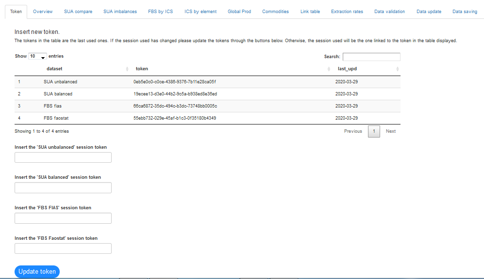
Figure 3.1: First tab appearing when opening the shiny app.
Note: ALL the tables displayed in the shiny app can be downloaded in CSV, Excel and PDF formats using the buttons showing the formats.
3.1 Token tab
The first tab, the ‘Token’ tab, allow the user to connect to the sessions compiled with the plugin. Each session created into the SWS has an identifier called token that allows the software R to connect and read data from the system. Since data computed by the plugin are not saved in the dataset but only in the session the user has to retrieve the session token to connect the shiny to the SWS. The needed tokens are those of the SUA unbalanced, the SUA balanced, the FIAS standardized FBS and the Faostat standardized FBS. In order to get the tokens the user must enter into the SWS select the ‘Run plugin’ button, select the ‘get_Token’ plugin and press the ‘Get debug token’ button. A window will open and the user can now copy and paste the token in the corresponding boxes in shiny app (figure 3.2) and save it pressing the ‘Update token’ button. The steps to obtain the token are described in figure @ref(fig:get_Token).
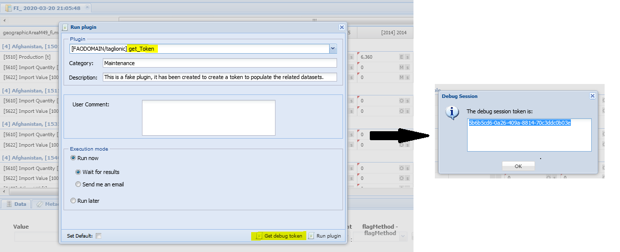
(#fig:get_Token)Example for the get token plugin.
This operation has to be done only when the plugin has just run and has provided new results, the shiny app stores the tokens into a SWS data table (‘fi_sua_fbs_token’) along with the date of the token update.
Even if the Faostat FBS is not used directly in the shiny it is updated along with the other dataset at the end of the process. A token is therefore needed for it as well. The ‘Data saving’ tab is similar to this one so a session needs to be created and the tokens saved for the correspondent validated datasets. Tokens of the validated datasets will be inserted into the ‘Data saving’ tab.
Note: the session with the plugin results cannot be deleted otherwise all the figures will be lost.
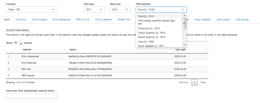
Figure 3.2: Overview of the Token tab.
After the user made sure the shiny app connects to the required sessions, the country, time period and FBS elements to visualize in the next tab can be selected (figure 3.2). The shiny app is conceived to work country by country as with the previous methodology.
3.2 Overview tab
Figure 3.3 presents the overview panel with the example of FBS results for Chile in the time period 2010-2017.
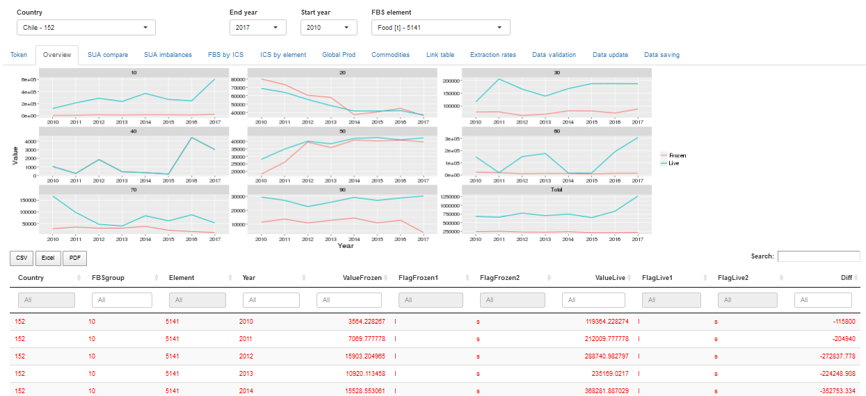
Figure 3.3: Overview of the Overview tab.
The tab has two parts: the graph part and the table part. In the graph part shows the time series for the chosen element (food in the example) of each major group plus the grand total. The graphs show the plugin results in light blue (Live, i.e. values saved in the FIAS FBS session) and the previously validated results in light red (Frozen, i.e. results saved in the FIAS FBS validated dataset). In this way the user can see what has been validated in the past and compare with the new results. The table underneath shows the figures corresponding to the time series in the graphs. The user can sort and filter data in the table as wished.
3.3 SUA compare tab
In the second tab the user has the comparison between ‘live’ and ‘frozen’ data for SUAs(figure 3.4). The user can select from the left-side menu what FBS group(s) and elements to visualize. For the elements an ‘Element group’ button has been created t allow the user to rapidly select several elements at the same time. The groups correspond to the following element choices: - Single: is the default choice, no element automatically selected, the user has to choose manually. - All: all elements are automatically selected. -Primary: only SUA unbalanced elements are selected, i.e. the production, import, export and also the input as it can reveal further details with respect to production only. -SUA: all the SUA elements, nutrition factors excluded. - Nutrients: only nutrient related elements are selected (Kcal/year, Kcal/caput/day, Proteins/year, Proteins/caput/day, Fats/year, Fats/caput/day).
From the table the user can sort and filter data and see the difference between the frozen and live data looking at the last table column ‘Diff’.
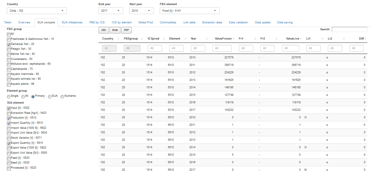
Figure 3.4: Overview of the SUA compare tab.
3.4 SUA imbalance tab
The SUA imbalance tab (figure 3.5) only reports SECONDARY imbalances. The reason is that the plugin does not fix primary imbalances, they are temporarily balanced with the Residual element (5166). They can be checked both in the ‘SUA compare’ tab and in the ‘Data validation’ tab, but the user has to manually fix with ad-hoc measures primary imbalances. Secondary imbalances are fixed by the plugin by increasing production figures until the imbalance is covered. FIAS unit required secondary products do not include meals that need ad-hoc solutions. They are therefore treated as primary products.
The tab has three part, the first up left parts has graphs of the imbalances by products. The user can see the series of imbalances and check the figures in the table in the up right part.
The table in the bottom part contains the production elements for all the SUAs (not only for secondary elements) and both original production and production after the increase are displayed. By giving this information the user controls and is aware of the increase and can modify the production figure in the ‘Data validation’ tab if needed.
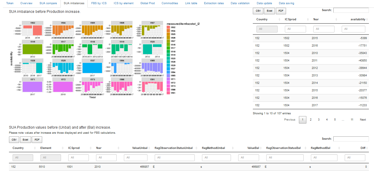
Figure 3.5: Overview of the SUA imbalance tab.
3.5 FBS by ICS tab
In order to have a more comprehensive vision of the composition of each FBS group, the ‘FBS by ICS’ tab gives the time series of each FBS element for all products composing the major group selected.
Because the shiny app takes values from the SUAs only values present both in the SUA and in the FBS can be checked. The graphs shows only products having data for the selected element. The table below shows the complete SUA for the selected group, the user can sort and filter the data in the table as usual.
Figure @ref{fig:shinyICS} shows the example of ‘Food (5141)’ for ‘Demersal fish (20)’ major group. From the left-side menu the user can select and deselect ICS products as wished.
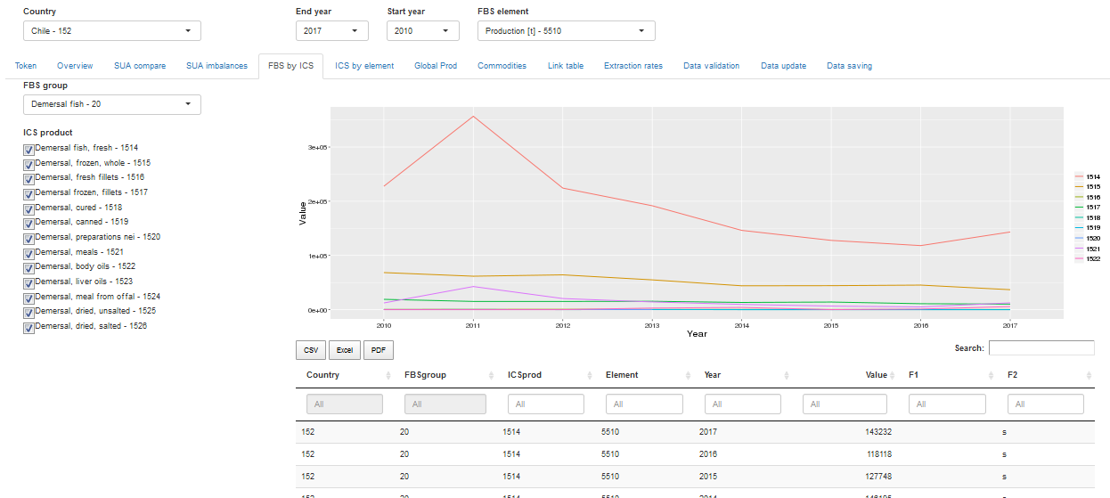
Figure 3.6: Overview of the FBS by ICS tab.
3.6 ICS by element tab
This tab allow the user to see, for the selected product, the time series of all SUA elements. From the left-side menu (figure 3.7), the user selects the major group and the product and then, by default, all the elements are shown in the graph along with the data in the table below. The user can select or deselect elements as wished.
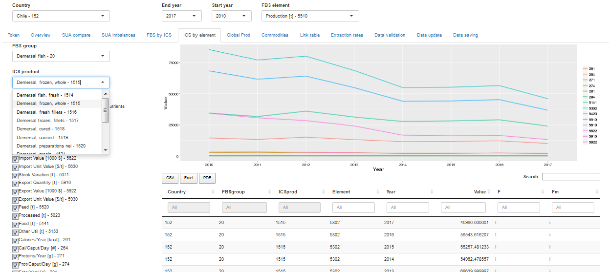
Figure 3.7: Overview of the ICS by element tab.
3.7 Global Production tab
In order to check data until the very first source, the user can look at the data in the Global production and the Commodity datasets respectively in the ‘Global prod’ and the ‘Commodities’ tabs. ‘Global prod’ tab (figure 3.8) allows the user to select one or more FBS group/s and to see all the species contained into the Global production dataset belonging to the selected group/s.
On the left-side part, in addition to the FBS group button, there is a table containing the deviation previously set for species in the selected country and allows the user to add a new deviation. The table is partially pre-compiled so that the user has to add only the species to deviate and to write from which ICS to what other one. Nevertheless, the user can always change the pre-compiled fields and change the validity period and the ratio. The validity period is set by default from the last year until the ‘LAST’ i.e. forever until a further modification is done. The ratio is 1 by default, but the user can split the quantity and deviate only a part of the production to a different product. In case the user wants to change destination only for one part, e.g. 40% and leave the other 60% to the original product, then only one row can be inserted, the 60% unchanged percent will automatically stay to the original ICS. If all the quantity has to be deviated to more than one product then all these alternative products must be specified. After the table has been modified it has to be saved into the SWS by clicking the ‘Save’ button in the upper-left part of the screen. This information is saved in a data table, meaning there is no further saving required. Differently from datasets, data tables are modified and saved directly from the shiny app with no other action to be done directly in the system.
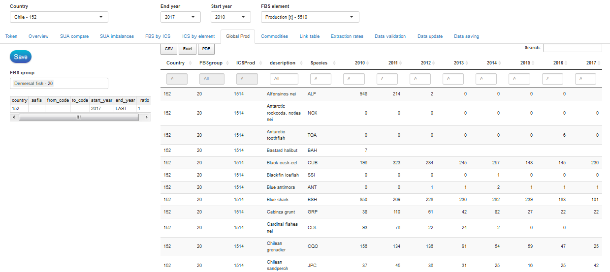
Figure 3.8: Overview of the Global production tab.
3.8 Commodities tab
The ‘Commodities’ tab is similar to the previous ‘Global prod’ tab but it also includes the possibility to select the specific ICS product (all the Global Production data are primary products so there was no need to add the ICS button). Also in this tab, there is the table for deviation of single commodities from one product to another and the user can complete and modify it the same way as described for the previous tab. The additional feature is the need to specify the flow to deviate as in the Commodity dataset there are also trade data, in addition to production. The user has to write the code of the element to deviate as displayed in the left-side menu and in the table (figure 3.9).
After the table has been modified it has to be saved into the SWS by clicking the ‘Save’ button in the upper-left part of the screen. This information is saved in a data table, meaning there is no further saving required. Differently from datasets, data tables are modified and saved directly from the shiny app with no other action to be done directly in the system.
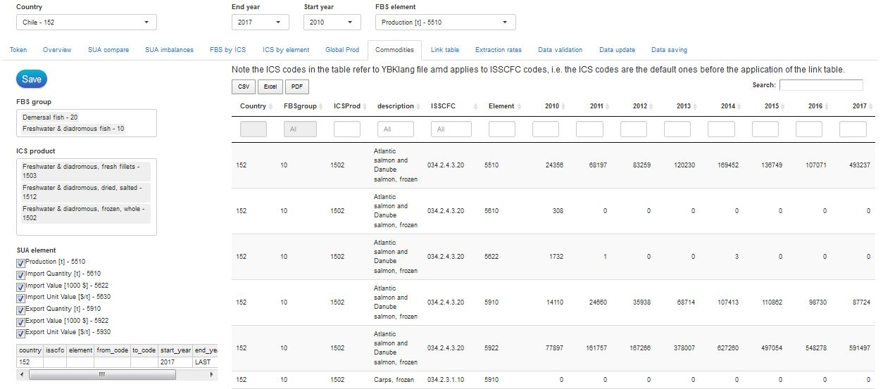
Figure 3.9: Overview of the Commodities tab.
3.9 Link table tab
Sometimes flows have to be deviated as a whole from one ICS product to another. For this reason the ‘Link table’ tab (figure 3.10) contains the table for the selected country and shows all the deviations already applied. The user can modify the table directly in the shiny app taking care to consistently insert the new information: write the flow with the same letters are other deviations and in capital letters: ‘PRD’ for production, ‘EXP’ for export, ‘IMP’ for import, ‘TRD’ for trade and ‘ALL’ for all flows; write the percentage in decimals (1 for 100%, 0.6 for 60%…).
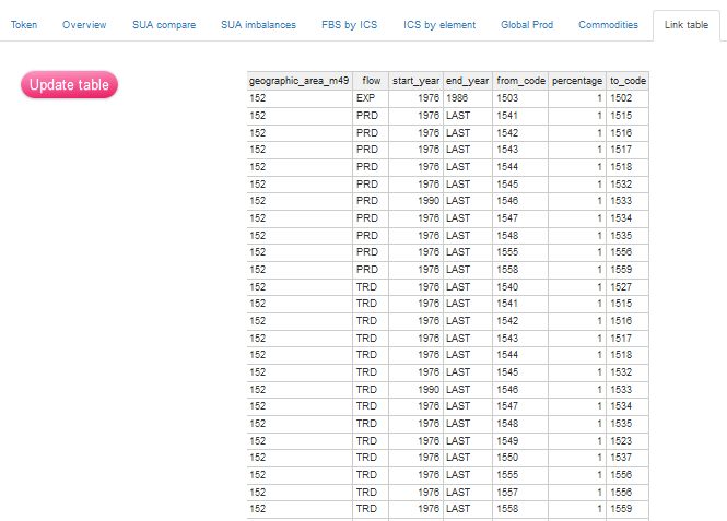
Figure 3.10: Overview of the Link table tab.
3.10 Balancing Elements tab
This tab has similar structure to the ‘link tab’ but it refers to balancing elements. If there is a new product or the balancing element needs to be changed, the user can do it directly from the shiny respecting the structure of the datatable as in figure 3.11.
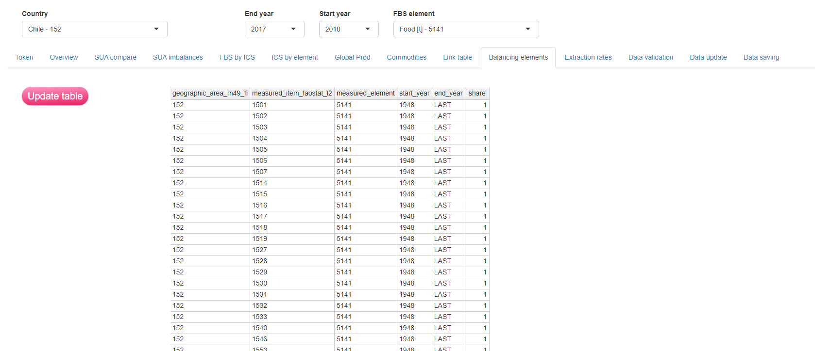
Figure 3.11: Overview of the Balancing elements tab.
3.11 Extraction rates tab
The ‘Extraction rates’ tab has been requested to perform block or single extraction rate updates and not to make year and product detailed operations. It has been conceived as a way to do updates that applies to more than one cell avoiding changing cells one by one. In this tab, figure 3.12, the user can change the figures for the extraction values and see the current values for the time series selected. Depending on the choice the user makes selecting the ‘Update type’ from the left-side menu, the modification can apply to single years or to the selected time series. Once the modification is validated (‘Update’ button in the left-side menu), the new figure appear in the ‘Data validation’ tab and will be applied during the new recalculations.
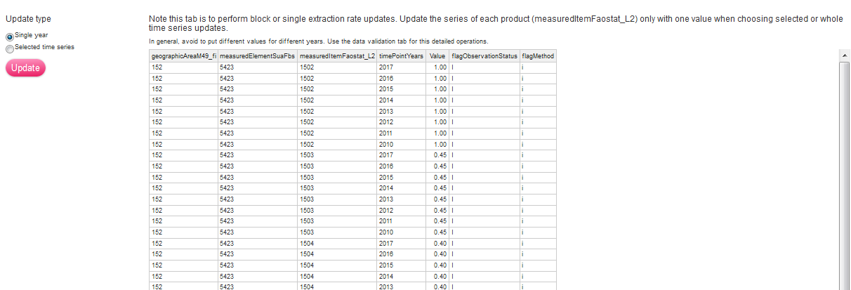
Figure 3.12: Overview of the Extraction rates tab.
3.12 Data validation tab
The data validation tab is the most interactive and the only true working tab of the shiny. From the left-side menu the user has to select the major groups, the products and the elements to visualize SUA for. The modification can be done in two ways:
- Directly on the tab
- Uploading a CSV file (CAUTION!)
In the case of file uploading the advice is to first download the whole SUA in CSV format, to modify figures in this file and to upload this same file which has already the right template to be processed by the shiny. Depending on the user’s choice the ‘Update to consider’ button must be selected accordingly.
The button to download and upload the file are in the upper part of the tab, figure 3.15. The user is allowed to do different kind of modification and, depending on them, to perform different kind of recalculations. First of all many changes concern extraction rates or the insertion of input values coming from publications. For this reason in the left-side menu (figure 3.14) the user has to choose if the recalculation functions have to prioritize the extraction rate or the input. If no official input is available then the better solution is to choose to use the extraction rate. If official input is available from publications, then the user can choose to prioritize the input so that the functions recalculate the extraction rates and flag the input as an official figure from publication. Note that the user has to choose one of the two in order to proceed to the reprocessing. Otherwise the shiny will return a message reminding to choose one option (by default the invalid ‘Null’ option is selected).
The user can choose to change some quantities and leave the others be recalculated freely from the functions or to assign all the quantities and define the exact form of the SUA balanced. Depending on the modification the user can also choose what kind or reprocessing the shiny has to perform:
If modifications involve Global production, Commodity or ICS deviations then a ‘Complete’ recalculation is the right choice and, in general, is the one that avoid any unwanted inconsistency.
If the user only wants to test the effect of a minor change only to see the effect on the SUA, then the ‘Only SUA balance’ choice is the quickest option.
If the user wants to recalculate from the SUA balanced until the FBS then ‘Since SUA balanced’ is the right choice.
If the user do not want the shiny to do any change to the SUA but only perform the aggregation and the nutrient related calculations, the ‘Only Nutrients & FBS’ button has to be selected.
After having selected all the options the button ‘Save and Recalc’ initiate recalculations and a window will notice when calculations are complete. After the end of the reprocessing calculations the new SUA appears in the tab and the effect on the FBS can be checked in the following tab.
The user can recalculate as many times as wanted bearing in mind each recalculation is saved and new calculations use the new calculated values.
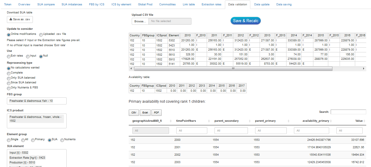
Figure 3.13: Overview of the Data validation tab.
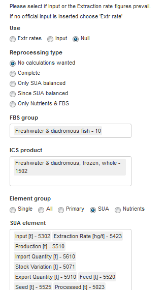
Figure 3.14: Side manu of the Data validation tab.
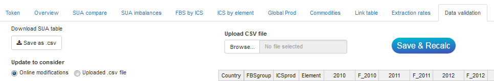
Figure 3.15: Upper part of the Data validation tab.
3.13 Data update tab
The ‘Data update’ tab is a copy of the ‘Overview’ tab but shows the FBS resulting from the recalculations of the previous tab. The user can compare the results (example in figure 3.16) with the ‘Overview’ tab that keeps on storing the original values and decide if to validate and save back this new SUA and FBS back into the SWS. If the user is satisfied of the results,or just do not want to lose the work so far the data have to be saved int the following tab and transfer all the figures for the country to the SWS.
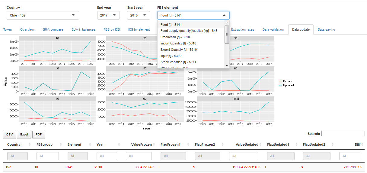
Figure 3.16: Overview of the Data update tab.
3.14 Data saving tab
This last tab is similar to the first tab ( Token tab) but the required tokens refer to the validated datasets corresponding to the modified datasets (figure @ref{fig:shinysave}). As with the other tokens the user needs to save them only once and they sessions will be saved. Once the user is satisfied with the modifications and does not need the previous data anymore the new values can be saved through the button ‘Update SWS’. The shiny will update BOTH the working sessions and the validated sessions so when restarting the work the user can start form where he/she was. In the unlikely (impossible?) case a non-reversible error is committed somehow and initial data cannot be retrieved the user can always re-run the ‘fi_SUA-FBS’ plugin for the country he/she lost data for.
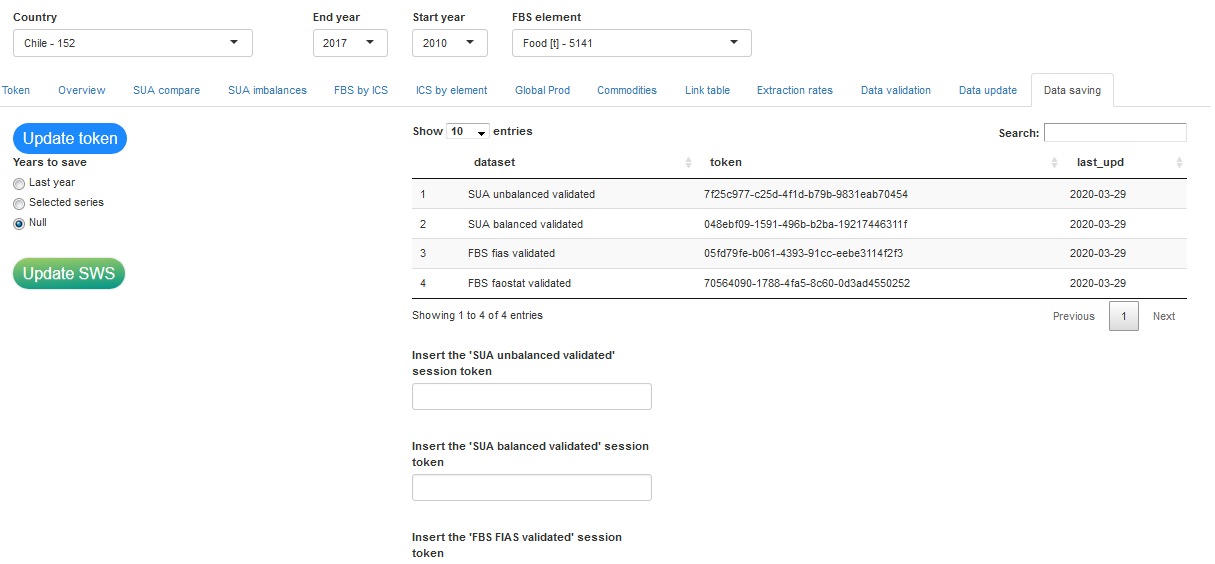
Figure 3.17: Overview of the Data update tab.
A message after the saving of all the dataset will notify the user the process has run correctly. It is important that after the update the user checks that the values have been saved in the session of the validated datasets and, ONLY when the final result are ready for the country, the data are saved from the session to the dataset.