Chapter 4 The aggregation module
The first part of the processed production data workflow focuses on national products classified according to scheda codes, whereas the Commodity dataset contains data classified according to the International Standard Statistical Classification of Fishery Commodities (ISSCFC). The connection between the codes is not an issue because, since the first upload into the SWS in the processed_prod_national_detail_raw data table, each scheda is linked to an ISSCFC code. This means the data table contains all the needed information for aggregation, as to each ISSCFC code corresponds to one or many scheda code. The aggregation process is two fold, it involves the value aggregation and the flag aggregation.
The value aggregation is simply the sum of all the value with the same ISSCFC code by country and year. Flag aggregation requires a more delicate process implemented according to FIAS requirements1. The rules applied for flag aggregation from the processed_prod_national_detail_imputed data table to the Commodity dataset are:
If the official value is more than the sum of (estimated + imputed) then the flag becomes official.
If the flag is not official, then allocate the flag of the maximum between estimated and imputed.
Else, keep the ranking used for N, O, M.
The ranking used for flag is in increasing order ‘M’, ‘O’, ‘N’, ‘’, ‘X’, ‘T’, ‘E’, ‘I’, meaning that ‘I’ is the strongest and ‘M’ the weakest in case of aggregation.
Because the first part of the workflow in the Statistical Working System (SWS) only involves data tables and does not use datasets, all the ISSCFC codes in the data table processed_prod_national_detail_imputed need a check. If all the codes are correct and exist in the ‘measuredItemISSCFC’ dimension they can be introduced into the Commodity dataset. The SWS only populates a dataset if all the codes exist in the dataset dimension.
4.1 The code
The aggregation plugin ‘fi_ProcProd2CommodityDB’ can be applied to a session or to the whole dataset. The parameters at the beginning of the process enable the user to choose between session country(ies) or all countries and between session years or all years.
##' # National processed production aggregation process for the Fishery commodity database
##'
##' **Author: Charlotte Taglioni**
##'
##' **Description:**
##'
##' This module is designed to aggregate processed production
##' products classified at national level into the ISSCFC.
##'
##' **Inputs:**
##'
##' * Processed prodution datable: processed_prod_national_detail_imputed


## Load the library
suppressMessages({
  library(faosws)
#  library(faoswsUtil)
  library(data.table)
})

# Token QA
if(CheckDebug()){

  library(faoswsModules)
  SETTINGS = ReadSettings("sws.yml")

  ## If you're not on the system, your settings will overwrite any others
  R_SWS_SHARE_PATH = SETTINGS[["share"]]

  ## Define where your certificates are stored
  SetClientFiles(SETTINGS[["certdir"]])

  ## Get session information from SWS. Token must be obtained from web interface
  GetTestEnvironment(baseUrl = SETTINGS[["server"]],
                     token = SETTINGS[["token"]])

}

#-- Parameters ----

dataInterest <- swsContext.computationParams$dataInterest
yearInterest <- swsContext.computationParams$yearInterest

if(is.null(dataInterest) | is.na(dataInterest)){
  stop('Please choose the data of interest.')
}

if(is.null(yearInterest) | is.na(yearInterest)){
  stop('Please choose the year(s) of interest.')
}

#-- Processed production loading ----

if(dataInterest == 'Selected country/ies and year(s)' & yearInterest == 'session'){
# country <- swsContext.computationParams$country
# start and end year for standardization come from user parameters
country <- paste("'",swsContext.datasets[[1]]@dimensions$geographicAreaM49_fi@keys, collapse = ",", "'")
country <- gsub(" ", "", country)
yearVals <- swsContext.datasets[[1]]@dimensions$timePointYears@keys
where <- paste("geographicaream49_fi in (", country, ")", sep = "")
procprod <- ReadDatatable('processed_prod_national_detail_imputed', where = where)
procprod <- procprod[timepointyears %in% as.character(yearVals), ]

} else if(dataInterest == 'All countries' & yearInterest == 'session'){

  yearVals <- swsContext.datasets[[1]]@dimensions$timePointYears@keys
  procprod <- ReadDatatable('processed_prod_national_detail_imputed')
  procprod <- procprod[timepointyears %in% as.character(yearVals), ]

}else if(dataInterest == 'Selected country and years' & yearInterest == 'all'){

  country <- paste("'",swsContext.datasets[[1]]@dimensions$geographicAreaM49_fi@keys, collapse = ",", "'")
  country <- gsub(" ", "", country)
  where <- paste("geographicaream49_fi in (", country, ")", sep = "")
  procprod <- ReadDatatable('processed_prod_national_detail_imputed', where = where)

} else {

  procprod <- ReadDatatable('processed_prod_national_detail_imputed')

}


# Delete unnecessary columns
procprod <- procprod[ , c("nationalquantity", "nationalquantityunit",
                          "id_isscfc", "nationalcode", "nationaldescription", "remarks",
                          "id_nationalcode", "measureditemnational") := NULL]

# set names according to the commodity dataset
setnames(procprod, c("geographicaream49_fi", "measuredelement", "timepointyears",
                     "measureditemisscfc", "quantitymt", "flagobservationstatus",
                     "flagmethod", "approach"),
         c("geographicAreaM49_fi", "measuredElement", "timePointYears",
           "measuredItemISSCFC", "Value", "flagObservationStatus",
           "flagMethod", "approach"))

message('fi_ProcProd2CommodityDB: Processed production datat loaded')
Once the parameters have been selected and the data loaded, all the columns that do not correspond to a dimension of the Commodity dataset are dropped. The ISSCFC codes check is performed and data aggregation process starts.
# Take columns of interest
dataFile <- procprod[ , .(geographicAreaM49_fi, measuredElement, timePointYears,
                          measuredItemISSCFC, Value, flagObservationStatus, flagMethod)]

# Get the dimension
isscfc <- GetCodeList(domain = 'FisheriesCommodities', dataset = 'commodities_total',
                      dimension = 'measuredItemISSCFC')[ , code]

# Check all ISSCFC codes belong to the dimension 'measuredItemISSCFC'
if(!all(dataFile$measuredItemISSCFC %in% isscfc)){
  stop(paste0('Code(s):', dataFile[!measuredItemISSCFC %in% isscfc], 'do(es) not belong to the measuredItemISSCFC dimension.'))
}

dataFile$Value <- as.numeric(dataFile$Value)
Data values are aggregated first according to country, element, year, ISSCFC and flag (dataFilebyflag) and then without considering flags and assigning by default the strongest flag (dataFilebyISSCFC).
# Take all values by flag to impute the right observetion flag
dataFilebyflag <- dataFile[ , list(Value = sum(Value, na.rm = TRUE)), by = c("geographicAreaM49_fi", "measuredElement",
                                                                             "timePointYears", "measuredItemISSCFC",
                                                                             "flagObservationStatus")]

dataFile$flagObservationStatus <- ifelse(is.na(dataFile$flagObservationStatus), ' ', dataFile$flagObservationStatus)
dataFile$flagObservationStatus <- factor(dataFile$flagObservationStatus,
                                         levels = c('M', 'O', 'N', ' ', 'X', 'T', 'E', 'I'),
                                         ordered = TRUE)

# Calculate total value by ISSCFC
dataFilebyISSCFC <- dataFile[ , list(Value = sum(Value, na.rm = TRUE),
                                     flagObservationStatus = max(flagObservationStatus)), by = c("geographicAreaM49_fi", "measuredElement",
                                                                               "timePointYears", "measuredItemISSCFC")]
dataFilebyISSCFC[is.na(flagObservationStatus) , flagObservationStatus := ' ']

# Compare data by ISSCFC and Flags with data only by ISSCFC
mergedFile <- merge(dataFilebyflag, dataFilebyISSCFC, by = c("geographicAreaM49_fi", "measuredElement",
                                             "timePointYears", "measuredItemISSCFC"),
      suffixes = c("_byflag", "_total"), all=TRUE)
The comparison between the two aggregations is based on the ratio between the value aggregated by flag and the value aggregated only by ISSCFC. If the ratio is higher than \(50\%\), the flag corresponding to the higher value is assigned, replacing the previous one assigned according to the defined order. The flag method assigned by default is ‘-’; if the value is official (flagObservationStatus = ‘’) then the method flag is a sum ’s’ as it should be since they are values resulting from an aggregation; if the value was estimated (flagObservationStatus = ‘E’) the method flag is ‘f’; if the value is missing (flagObservationStatus = ‘O’ or ‘M’) then the method flag is kept as ‘-’.
# Calculate ratio
mergedFile[ , ratio := Value_byflag/Value_total]
mergedFile[ , ratiocheck := sum(ratio, na.rm = TRUE), by = c("geographicAreaM49_fi", "measuredElement",
                                                             "timePointYears", "measuredItemISSCFC")]
all(mergedFile$ratiocheck %in% c(0,1))

# If ratio over 0.5 then flag is the flag having more than 50% of data, other wise is the normal hierarchy that wins
mergedFile[!is.na(ratio) & ratio > 0.5 & flagObservationStatus_total != flagObservationStatus_byflag, flagObservationStatus_total := flagObservationStatus_byflag]

# flag method assigned consequently, i.e. flag combinations are: ( , -), (E, f), (O, -) or (M, -)
mergedFile[ , flagMethod := '-']
mergedFile[flagObservationStatus_total == ' ', flagMethod := 's']
mergedFile[flagObservationStatus_total == 'E', flagMethod := 'f']
mergedFile[flagObservationStatus_total %in% c('O', 'M'), flagMethod := '-']
Data are eventually prepared to fit the Commodity dataset requirements along with metadata. Metadata collect the information contained in the ‘approach’ column of the data table so that, even in the Commodity dataset, the user has information about how the data have been estimated.
# Data reshape
mergedFile[ , c("flagObservationStatus_byflag", "Value_byflag", "ratio", "ratiocheck") := NULL]
setnames(mergedFile, c("Value_total", "flagObservationStatus_total"), c("Value", "flagObservationStatus"))
mergedFile$flagObservationStatus <- as.character(mergedFile$flagObservationStatus)
mergedFile[flagObservationStatus == " ", flagObservationStatus := ""]
setkey(mergedFile, geographicAreaM49_fi, measuredElement, timePointYears, measuredItemISSCFC, Value, flagObservationStatus)

# File to save ready
data2save <- mergedFile[!duplicated(mergedFile)]
message('fi_ProcProd2CommodityDB: Data ready.')

#-- Metadata ----

# Approach used goes in the metadata
metadataFile <- procprod[ , .(geographicAreaM49_fi, measuredElement, timePointYears,
                              measuredItemISSCFC, approach)]
setkey(metadataFile)
metadataFile <- unique(metadataFile)

# Message
metadataFilePresent <- metadataFile[!is.na(approach) , list(approach = paste(approach, collapse = ', ')),
                                     by = c("geographicAreaM49_fi", "measuredElement",
                                            "timePointYears","measuredItemISSCFC")]
setnames(metadataFilePresent, 'approach', 'Metadata_Value')

# Metadata structure
metadata2save <- metadataFilePresent[, `:=` (Metadata = 'GENERAL',
                                       Metadata_Element = 'COMMENT',
                                       Metadata_Language = 'en')]

message('fi_ProcProd2CommodityDB: Metadata ready.')

save <- SaveData(domain = "FisheriesCommodities", dataset = 'commodities_total',
                 data = data2save, metadata = metadata2save, waitTimeout = 100000)

paste0("ISSCFC commodity aggregation completed successfully!!! ",
       save$inserted, " observations written, ",
       save$ignored, " weren't updated, ",
       save$discarded, " had problems.")

## Initiate email
from = "sws@fao.org"
to = swsContext.userEmail
subject = "Commodity dataset aggregation"
body = paste0("Data have been properly aggrergated from the source datatable. There have been: ",
              save$inserted, " observations written, ",
              save$ignored, " weren't updated, ",
              save$discarded, " had problems.")


sendmail(from = from, to = to, subject = subject, msg = body)

paste0("ISSCFC commodity aggregation completed successfully!!! ",
       save$inserted, " observations written, ",
       save$ignored, " weren't updated, ",
       save$discarded, " had problems.
       Plugin has sent an email to ", swsContext.userEmail)
The last part of the plugin sends an email to the user and reporting the number of values written, updated or discarded in the Commodity dataset.
4.2 Practical tips and final remarks
The first step is the Commodity dataset query figures 4.1 and 4.2.
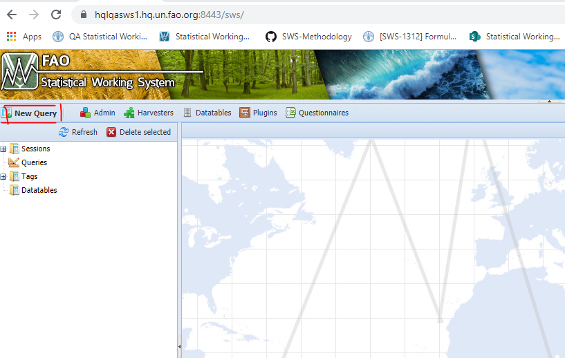
Figure 4.1: Commodity dataset query.
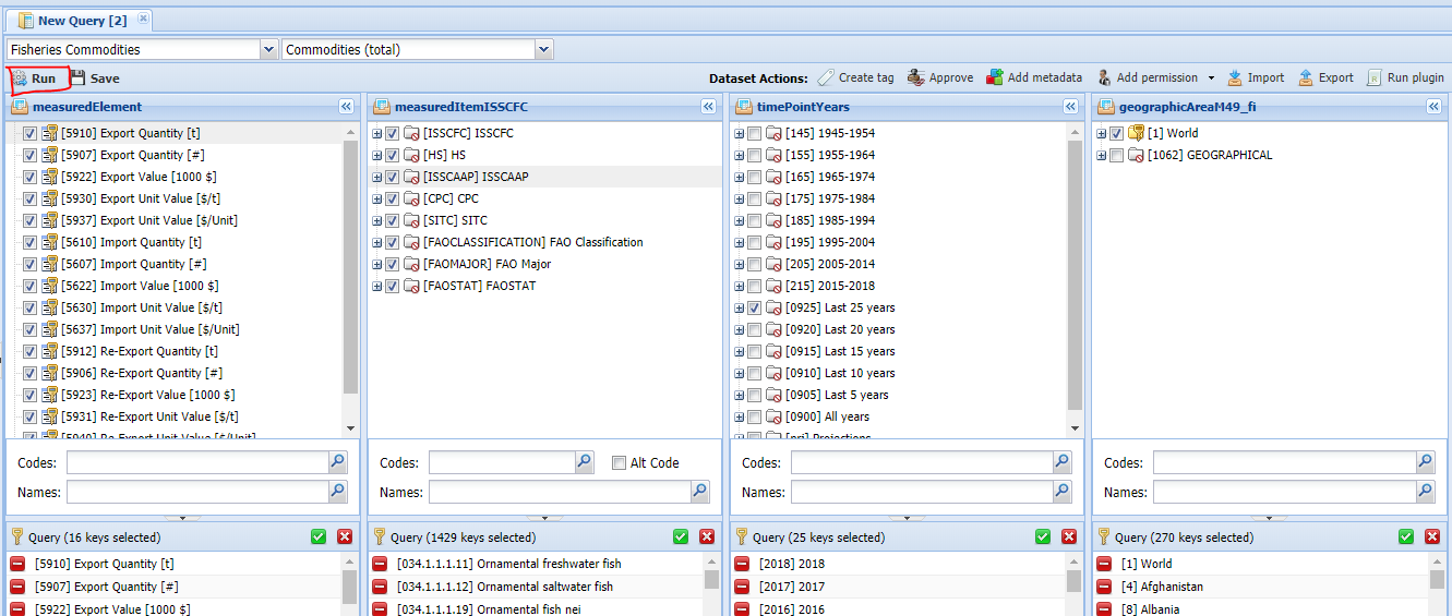
Figure 4.2: Commodity dataset query. Choosing dataset and dimensions
Once the session is open the plugin can be run selecting the ‘Run plugin button’ (figure 4.3), choosing the ‘fi_ProcProd2CommodityDB’ plugin (figure 4.4) and selecting the parameters (figure 4.5)
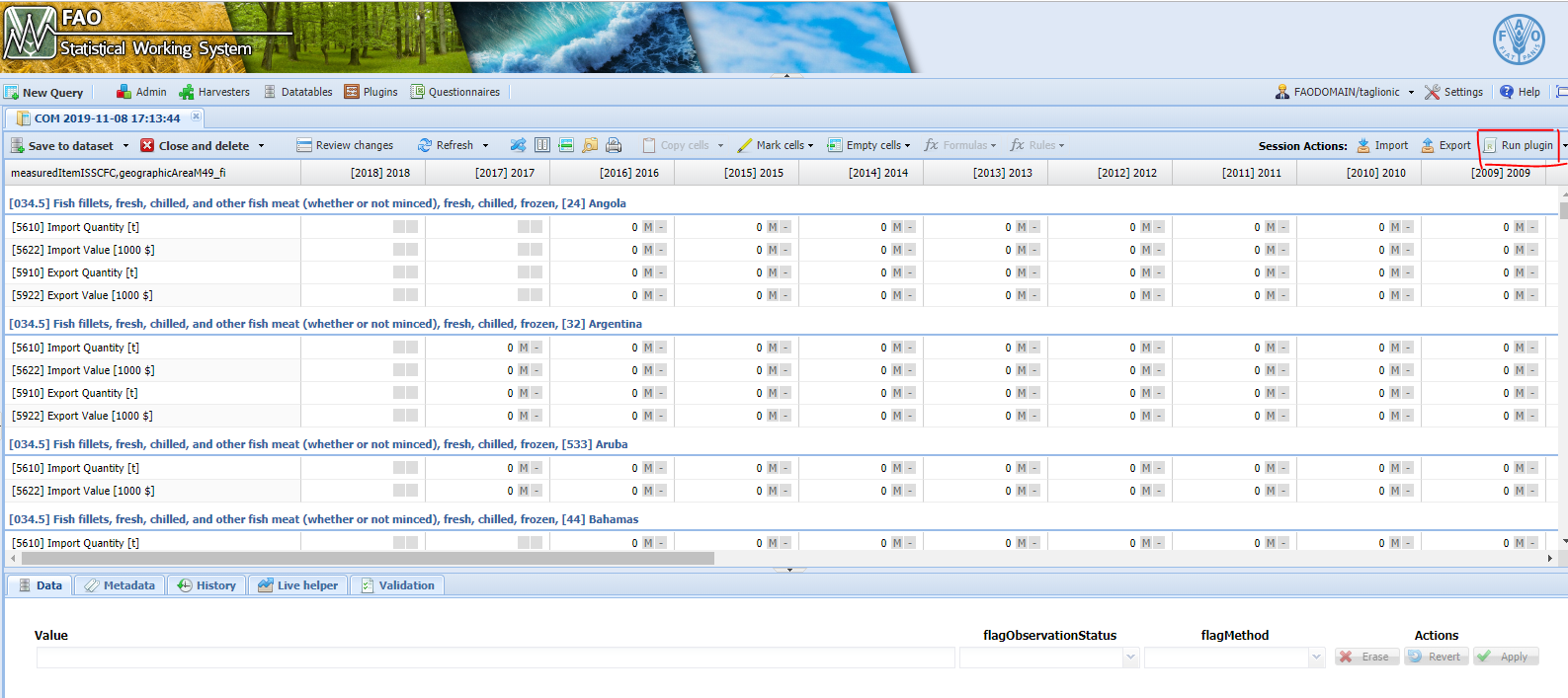
Figure 4.3: Run plugin
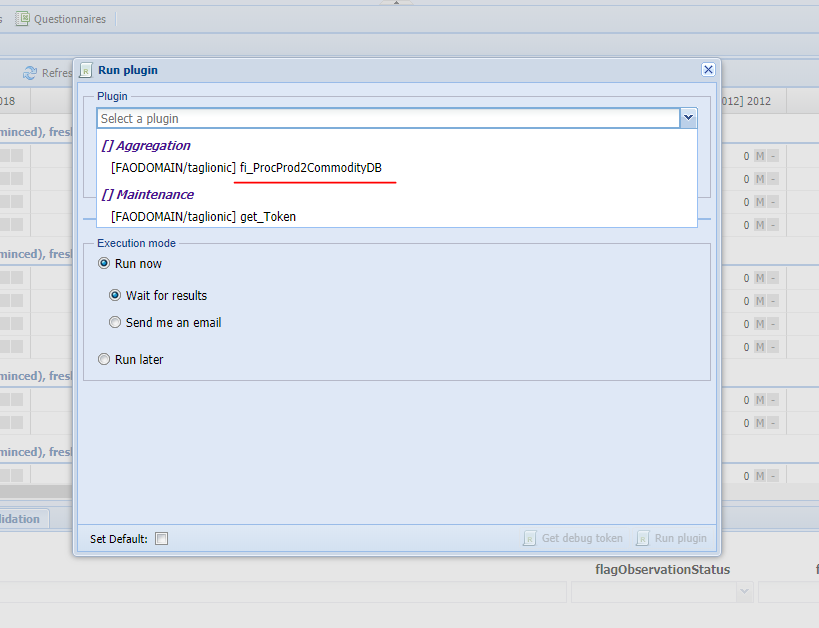
Figure 4.4: Selecting the fi_ProcProd2CommodityDB plugin.
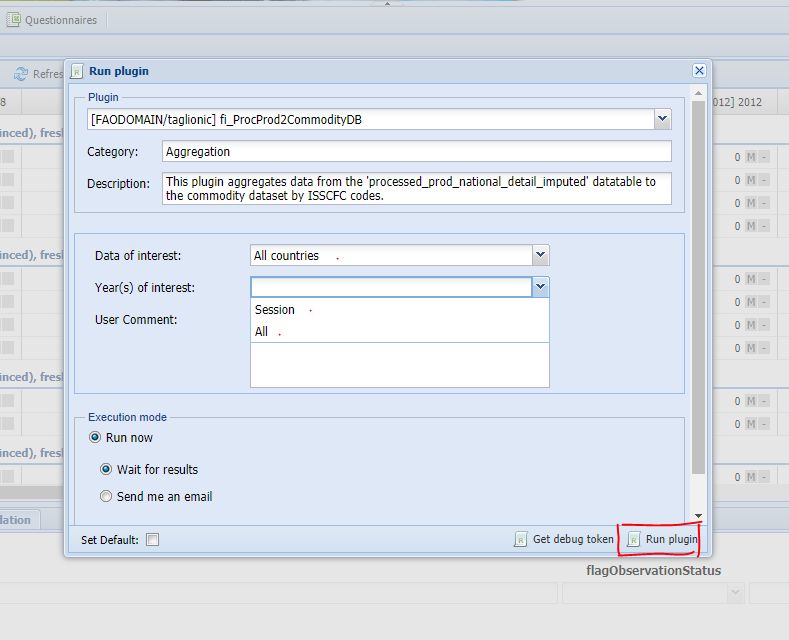
Figure 4.5: Selecting parameters and running the plugin.
After the plugin has run data have to be saved (‘Save to dataset’ button) and the Commodity dataset is complete with both processed production and trade data (the workflow requires trade data to be validated, aggregated and saved into the Commodity dataset before starting the processed production data process). Once the processed production data have been aggregated and saved into the Commodity dataset the process is complete and all the data are ready for use.
Email of August 8, 2019↩