4 Outlier Detection

The outlier detection is unlocked to be run only for the countries for which the imputation has been completed. Therefore, the input data is the data table fishtrade_data_imputed_validated under domain Fisheries Commodities. The main goal of the outlier detection in the Fisheries Module is to figure out discrepancies under the trade data. In the outlier detection process, we should be able to validate the outliers detected, once some values considered as anomaly can be part of the nature of the data. Besides, the methods should be flexible such way the user should be able to run the detection at different levels of aggregation:

• From the most aggregated one: All reporters / All Flows / All FAO major groups / All partners
• To the most detailed one: Reporter / Flow / Tariff line / Partner.

No matter the level of aggregation at which the detection is carried out, all modifications or corrections proposal are made at the most detailed level: Reporter | Flow | Tariff line | Partner. When the outlier detection is done at a higher level than the most detailed one (Reporter | Flow | Tariff line | Partner), the user can drill down in order to get to the most general level. When an outlier is identified at an aggregated level, then the tool propagates the correction to lower levels proportionally. Edits are done at the Reporter | Flow | Tariff line | Partner level. The fields that the user can edit are the quantity, the value, the flags and the remarks fields. The unit value and all of the aggregates can be recalculated on the fly after an edit in order to see the implications of the change. In Figure 4.1 is shown the workflow of the outlier detection module.

• Function: run_outlier_detection_module

Figure 4.1: Outlier Detection Flow.

4.1 Methods for outlier detection

In the Outlier Detection Module is applied two different methods. One that considers the data points as independent across the years, and another that takes account of the time correlation. The idea is to be able to find discrepancies when we compare one figure to the mass of data points, and the second one allows to check if the value is out of the data trend.

The outlier detection methods are applied in the unit value (uv), which is the ratio between the monetary transaction value and its weight, weight, and value variables. In this first step of this procedure, we attempt to figure out outliers in the aggregate level, and then we try to fix the transactions (disaggregated level) that were responsible for generating the outliers detected.

4.1.1 Boxplot rule

A boxplot is resource graphic to summarise a distribution of data based on a five numbers summary: “minimum”, first quartile (Q1), median, third quartile (Q3), and “maximum”. It allows us to visualise the outliers and their values. Also, if the data is symmetrical and how tightly your data is grouped. In Figure 4.2 is exemplified the five numbers summary.

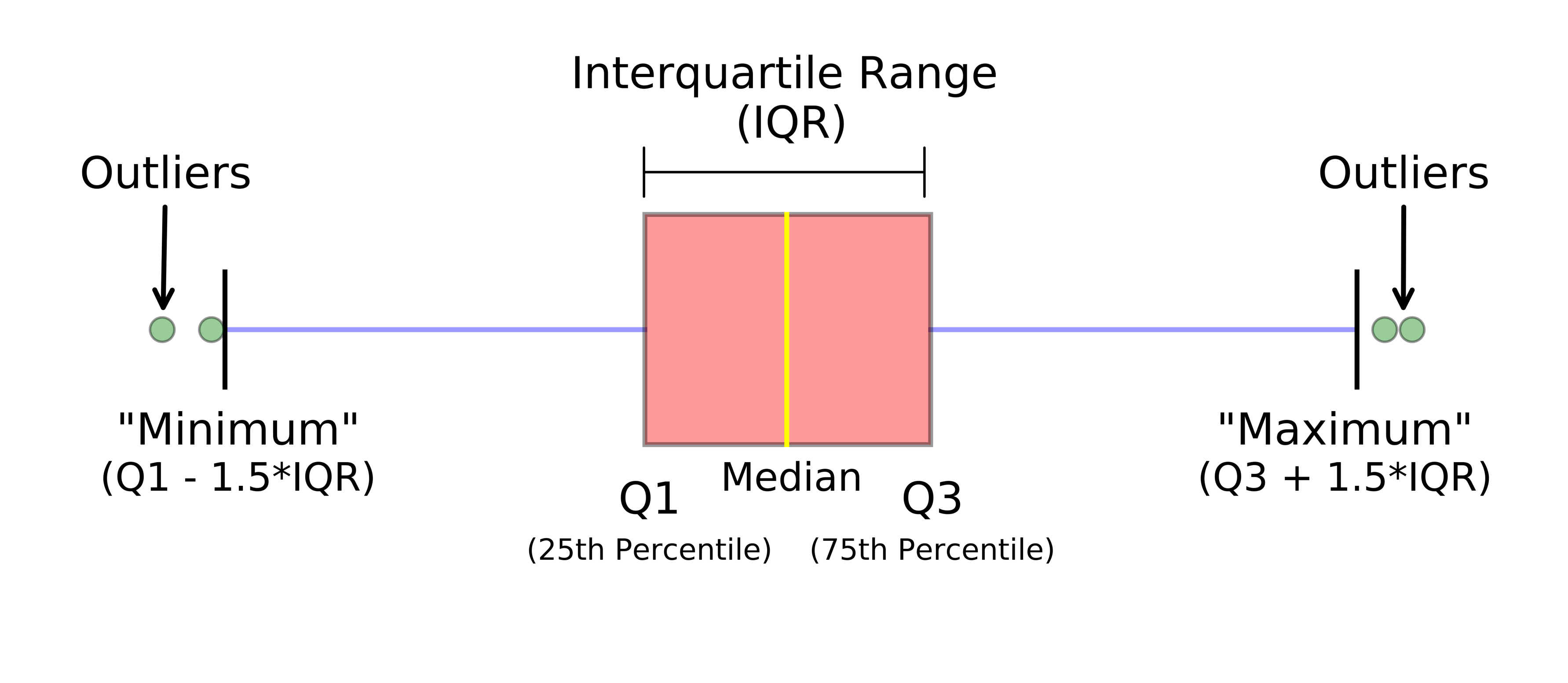
Figure 4.2: Example of a boxplot.
Source: https://towardsdatascience.com/understanding-boxplots-5e2df7bcbd51

The steps below aim to apply the boxplot rule in order to figure out discrepant values. Basically, the boxplot rule has an only parameter, \(k\), which is used to compute the upper and lower limits of the boxplot whiskers. In Figure 4.2 the parameter \(k\) is set equal \(1.5\), which is the value for the traditional boxplot.

1. Set the coefficient \(k\), for instance \(k = 5\).
2. Compute the percentiles: 25% (\(Q_1\)), and 75% (\(Q_3\)).
3. Compute the interquartile range (IQR): \(IQR = Q_3 - Q_1\)
4. Compute \(\text{limsup} = Q_3 + k \times IQR\)
5. Compute \(\text{liminf} = Q_1 - k \times IQR\)
6. If \(x > \text{limsup} \mid x < \text{liminf}\), then \(x\) is a outlier.

Note that there are no assumptions to use the boxplot. Nevertheless, it does not make sense to use the boxplot for small sample size. In this case, we added another parameter in Outlier Detection Module to tune the minimum sample size to apply this rule. Besides, it is known that the logarithmic function is useful to stable the data distribution, hence the user can choose to apply the logarithmic before to use the boxplot rule, which transforms the method more conservative, i.e., fewer values will be considered as outliers.

In Figure 4.3 is shown a screenshot of the Outlier Detection Module. Note that there is a dialog box to select which source the user wishes to apply the detection of outliers. This option allows the user to choose between the data table fishtrade_data_imputed_validated or fishtrade_outlier_corrected.

• Function: od_box_plot

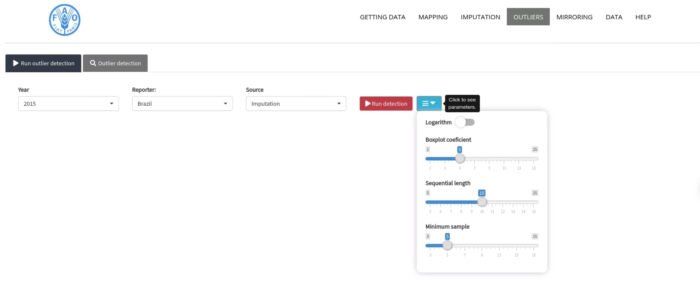
Figure 4.3: Outlier Detection Module: list of parameters to be used on this module.

Correction

Once the outlier has been detected, a correction is proposed automatically to be validated by the expert later. The method of correction for outliers detected through the boxplot is made by drawing randomly from a \(Uniform(a, b)\) distribution, where the limits of the distributions are:

Let be \(z\) a value detected as a outlier by the boxplot rule.

• If \(z < \text{minimum} \Rightarrow a = \text{minimum}\)
• If \(z < \text{minimum} \Rightarrow b = \text{median}\)
• If \(z > \text{maximum} \Rightarrow a = \text{median}\)
• If \(z > \text{maximum} \Rightarrow b = \text{maximum}\)

While the value is considered as an outlier, draws from Uniform distribution a correction proposal.

The idea behind this method is to trust that the outlier detected indeed is discrepant, but it is not too much great or small. Therefore, we select a value randomly from the half of the data distribution in order to “correct” this value. In Figure 4.4, we show a illustration of the boxplot correction.

Figure 4.4: Illustration of the boxplot correction..

4.1.2 Time Series

The Time Series method is applied only for those aggregations with more than \(s\) sequenctial years available. This parameter \(s\) is shown in Figure 4.3 as “Sequential length”. Another parameter is the logarithmic, the user can choose if it will be applied the logarithmic over the target variable or not.

The outliers are identified by fitting a loess curve for non-seasonal data and via a periodic STL decomposition for seasonal data. If the residuals, difference between fitted and observed values, lie outside the range \(\pm{2}(q_{0.9}-q_{0.1})\) where \(q_p\) is the \(p-\)quantile of the residuals, then they will be considered as outliers. For a Gaussian distribution, it will identify less than \(1\) point in \(3\) million as an outlier.

In Figure 4.5, we show an example of time series and its respectively loess curve fitted. Note that, the loess curve follows the data trend. In this example, it is easy to identify the outlier candidate. The next step is to compute the difference between the curves to get the residuals.

Figure 4.5: Time series of the data observed and the loess curve fitted.

In Figure 4.6, we show the histogram of the residuals as well as the limits used to identify the outliers. Note that, there is only one value that lies outside of the interval, hence this value is considered as outlier. The limits are defined as following:

1. Compute the quantiles \(q_{0.25}\), and \(q_{0.75}\).
2. Compute the interquartile range : \(IQR = q_{0.75} - q_{0.25}\)
3. Limits:
   • \(\text{liminf} = q_{0.25} - 3 \times IQR\)
   • \(\text{limsup} = q_{0.75} + 3 \times IQR\)

Figure 4.6: Histogram of the residuals and their respectively limits.

Correction

In the Time Series method, the correction is performed by replacing the values detected as outliers by fitted values. In Figure 4.7, we show how the correction is performed over the time series method.

• Function: od_ts_toolbox

Figure 4.7: Fitted values used as correction proposal.

4.2 Examples

The outlier detection methods are applied in the unit value (uv) variable, which is the ratio between the monetary transaction value and its weight. In this first step of this procedure, we attempt to figure out outliers in the aggregate level, and then we try to fix the transactions (disaggregated level) that were responsible for generating the outliers detected.

The aggregated level means to compute the unit value by reporter, flow, and FAO code, i.e., for each combination of reporter, flow, and FAO code we calculate the ratio between the summing of the monetary value and the summing of the weight. For instance, in Table 1 is shown a subset from the full data using the following parameters:

• reporter: 76
• year: 2005
• flow: 1
• faocode: 292.9.1.90

To calculate the unit value in the aggregate level, it is needed to apply the equation below:

\[uv = \frac{\sum_{p = 1}^{P} value_p}{\sum_{p = 1}^{P} weight_p}\] where \(value_p\) is the monetary value from the p-th partner, as well as \(weight_p\) is the transaction weight, \(P\) is the total of partners in this given combination, in this small example \(P = 12\). In order to make this report comprehensible, we show the uv calculation step-by-step as following:

\[\begin{align} uv & = \frac{65438+1910 + \cdots + 44329+438234}{73173+613 + \cdots + 5949+93719} \\ \\ & = \frac{1,893,528}{1,805,531} \\ \\ & = 1.05 \end{align}\]

If we repeat it procedure for all available year for this combination, we will find the values shown in Table 2. The highlighted row shows the uv computed previously, as shown in the equations sequence.

In Figure 1 is shown the same information stored in Table 1, i.e., the unit value computed in the aggregated level by year. The outlier can be easily identified when we look to the graphic below. The uv seems to be a stable behavior from 2000 to 2011 when you analyze Figure 1. However, in 2012 a sharp increase in the uv is noted. On the other hand, when we look at Figure 2, that is the same information, but without the year 2012, so it is possible to see clearly the increasing trend starting in 2007.

Figure 4.8: Figure 1: The whole time series of imports.

Figure 4.9: Figure 2: The time series of imports without the year 2012.

Despite the visual approach works well to identify the possible outliers, it is not possible to check each graphic to figure out the outliers. Therefore, it needs to use a general rule that can be applied in each combination. In the next section, we show two methods to figure out outliers in the trade data, the first one is the Boxplot, and the second one is the Median Absolute Deviation (MAD).

4.3 Boxplot

One of the methods to try figured out outlier in the aggregated data is the boxplot rule.

1. Set the coefficient \(k\), for instance \(k = 5\).
2. Compute the percentiles: 25% (\(Q_1\)), and 75% (\(Q_3\)).
3. Compute the interquartile range (IQR): \(IQR = Q_3 - Q_1\)
4. Compute \(\text{limsup} = Q_3 + k \times IQR\)
5. Compute \(\text{liminf} = Q_1 - k \times IQR\)
6. If \(uv > \text{limsup} \mid uv < \text{liminf}\), then \(uv\) is a outlier.

The IQR is a measure of variability, based on dividing a data set into quartiles. Quartiles divide a rank-ordered data set into four equal parts. The values that separate parts are called the first, second, and third quartiles; and they are denoted by Q1, Q2, and Q3, respectively.

4.3.1 Example

1. \(k = 5\)
2. Compute the percentiles:
   • \(Q_1 = 1.167\)
   • \(Q_3 = 1.788\)
3. \(IQR = Q_3 - Q_1 = 0.621\)
4. \(\text{limsup} = 4.893\)
5. \(\text{liminf} = -1.938\)

Figure 4.10: Figure 3: Boxplot exemplifying the outlier detection.

4.4 Locally Estimated Scatterplot Smoothing (LOESS)

To fix the transactions that generated the outlier in the aggregated level is fitted a LOESS model considering the log(uv) as variable response and year as the covariate. The rows which the year was detected as outlier were removed before to fit the model. Once the model is fitted, it is used to predict a new value to the given year. In our example, the year is 2012 and the value predicted by model is 4.701.

4.4.1 Example

Figure 4.11: Figure 4: Correction of the outlier using the LOESS model.